580 California St., Suite 400
San Francisco, CA, 94104
This research theme addresses the development, validation, and comparison of numerical techniques for simulating water waves with a focus on enhancing accuracy and computational efficiency. It covers methodologies for imposing boundary conditions, wave generation in numerical tanks, and modeling complex wave behaviors through advanced discretization and turbulence modeling approaches. Such improvements are crucial for replicating realistic wave phenomena in engineering contexts including coastal engineering, ocean energy devices, and offshore infrastructure.
This theme encompasses numerical modeling of nonlinear effects in wave breaking, turbulent flow structures, and free surface tracking between air and water phases. It addresses the complexity of simulating breaking wave kinematics, turbulent energy production and dissipation, wave-induced pressures, and accurate capturing of interfaces in multiphase flows. Progress in turbulence closure models and high-order numerical schemes aiming to realistically replicate physical wave breaking processes is central to advancing coastal and ocean engineering simulations.
This research area focuses on developing exact or improved boundary conditions to isolate finite computational domains within unbounded fluid regions, particularly for wave motion over uneven seabeds and underwater structures. Methods such as Dirichlet-to-Neumann (DtN) conditions and boundary integral equations enable efficient domain reduction while maintaining accurate wave field solutions. Coupled with appropriate discretization techniques like cubic hyperbolic B-splines and differential quadrature methods, these approaches facilitate precise simulation of 3D wave propagation in complex coastal or offshore settings.
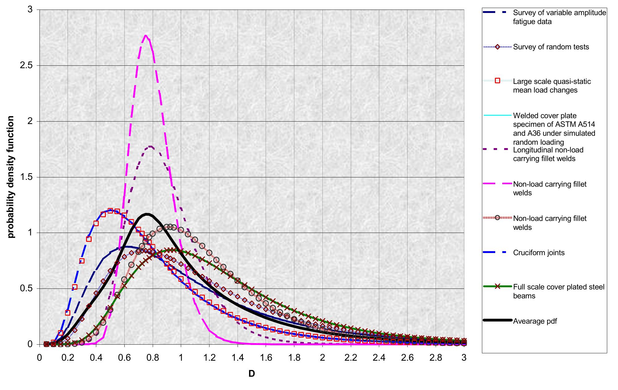
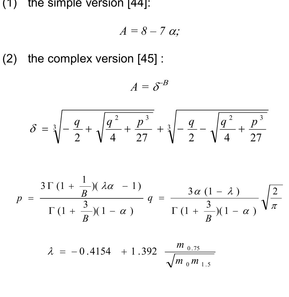
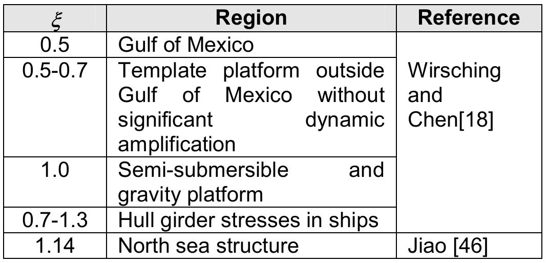
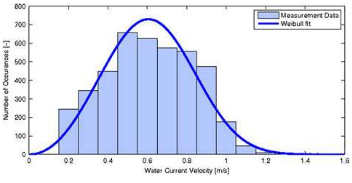
![Zhao and Baker proposed a combined distribution consisting of a Weibull and a Rayleigh distribution [44][45] as](https://figures.academia-assets.com/40498005/figure_003.jpg)
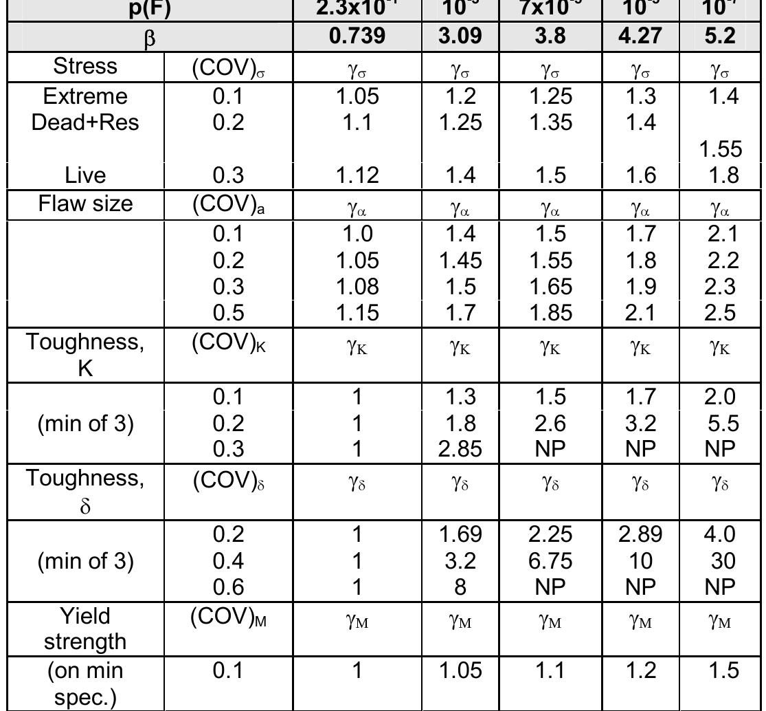
![Figure 3 Correspondence of the Master curve with the ASME Kj, data base (Sokolov [85]) Partial Safety Factor Approach for Fracture Assessment](https://figures.academia-assets.com/40498005/figure_007.jpg)
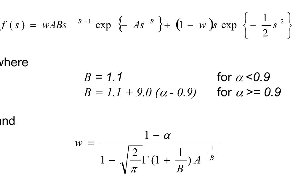
![Table 1: Percentage relative error using Paris law random variables This review concentrated on the probabilistic models for the randomised parametric approach. The deficiency in the randomised parametric approach was however noted by Proppe and Schuller [12] who compared fatigue prediction results by using the test data of Virkler [1] in randomised Paris and Forman’s aws. The parameters in the crack growth equations were obtained directly from the full dataset. They found that the relative errors in the mean values are relatively small but the errors in variances are quite arge, as seen in Table 1 for randomised Paris Law approach. Similar relative errors are found in randomised Forman’s law approach. They suggested he Markov chain models to be used to overcome this deficiency. Nguyen and Wirsching studied the combination of FORM and first passage theory [14] by using the exceedance rate from the Madsen [15] formula and approximating the probability of failure from curve fitting and integration.](https://figures.academia-assets.com/40498005/table_001.jpg)
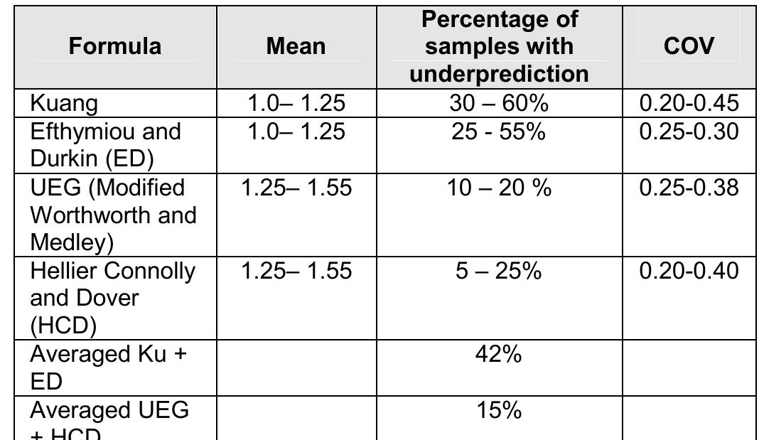
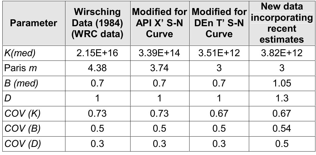
![Table 5: S-N uncertainty models Under the normal conditions defined for the S-N curves, Xu et al [33] specified the models in Table 5.](https://figures.academia-assets.com/40498005/table_003.jpg)
![where x;’ is the position, u;” is the velocity, p is the density, o,% is the total stress tensor, m is the mass and g;* is the gravitational force. The total stress tensor o; is made up from the isotropic pressure p; and the viscous stresses according to The governing equations for density and momentum evolution of the field for the multi-phase model are given by 12]](https://figures.academia-assets.com/48739046/figure_002.jpg)
![This Section presents the governing equations in SPH form. Throughout this paper, subscripts i and j denote the interpolated particle and its neighbours respectively. The density evolution and momentum of the particles follow the Navier-Stokes equations [16] where x; is the position , u; is the velocity , p is the density , P is the pressure, m is the mass and g; is the gravity acceleration. In this paper, the Wendland kernel [17] has been used as a smoothing function but numerical tests have shown similar](https://figures.academia-assets.com/48739046/figure_005.jpg)
![where p;, p; are respectively the density and the pressure of t a Bi t t t = he i—particle while r; and wu; are its position and velocity. he particle mass, m;, is constant during the motion so that he global mass i conserved exactly. Here, Wj; is the kernel function (a Wendland kernel is used hereinafter), V; denotes he differentiation with respect to r; and f; is the body force at he position r;. Finally, symbols pp and cp indicate the density along the free surface (which is the reference value for the density field) and the sound velocity (assumed to be constant). The dynamic viscosity is indicated through py while the kernel of the viscous term is given in [7] and reads: Hereinafter we call standard SPH the following system:](https://figures.academia-assets.com/48739046/figure_007.jpg)
![where subscript / and d refer to the liquid and dust, respectively, P is the pressure, K is a drag factor, v, and vg are the liquid and dust velocities, respectively, and g is the external self-gravity. 6; and fg are the effective densities of each phase per unit volume of the mixture, and are related to p, and pg, the material densities of each phase by The equations for continuum analysis we used are those given by Harlow and Amsden [6], [7] and continuity equation therefore has an extra sink term that can be interpreted in an SPH formulation by allowing the SPH dust particles to lose mass in the neighbourhood of the sedimenting boundary. This algorithm enables us to simulate the sedimentation in the presence of turbulence without resolving the thin boundary layer.](https://figures.academia-assets.com/48739046/figure_011.jpg)
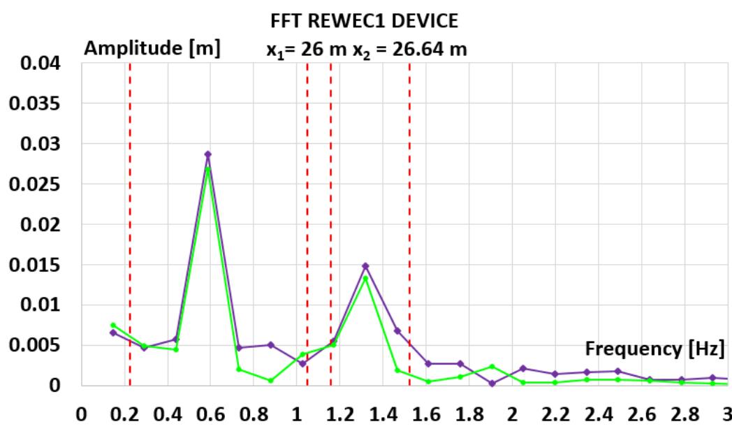
![Fig. 1 a) Conventional breakwater and, b) REWEC1 schematics breakwaters, Young and Testik [9] carried out experimental tests with both vertical and semi-circular barriers. It is observed that the reflection coefficient mainly depends on the ratio between the submergence of the structure, a, and the height of incident wave, H;. This allows one to obtain two semi-empirical parametric expressions of the reflection coefficient in the case of both vertical and semi-circular breakwaters. For the same values of the ratio a/Hj,, vertical structures reflects more energy than semi-circular structures. The reflection coefficient can also be obtained by means of calculation methods, which allow the separation of the reflected and incident wave components. These methods can be divided into two categories: methods operating in the time domain and methods operating in the frequency domain. In this work, the method proposed by Kittitanasuan & Goda [10], which belongs to the second category, has been taken into account.](https://figures.academia-assets.com/41855919/figure_001.jpg)
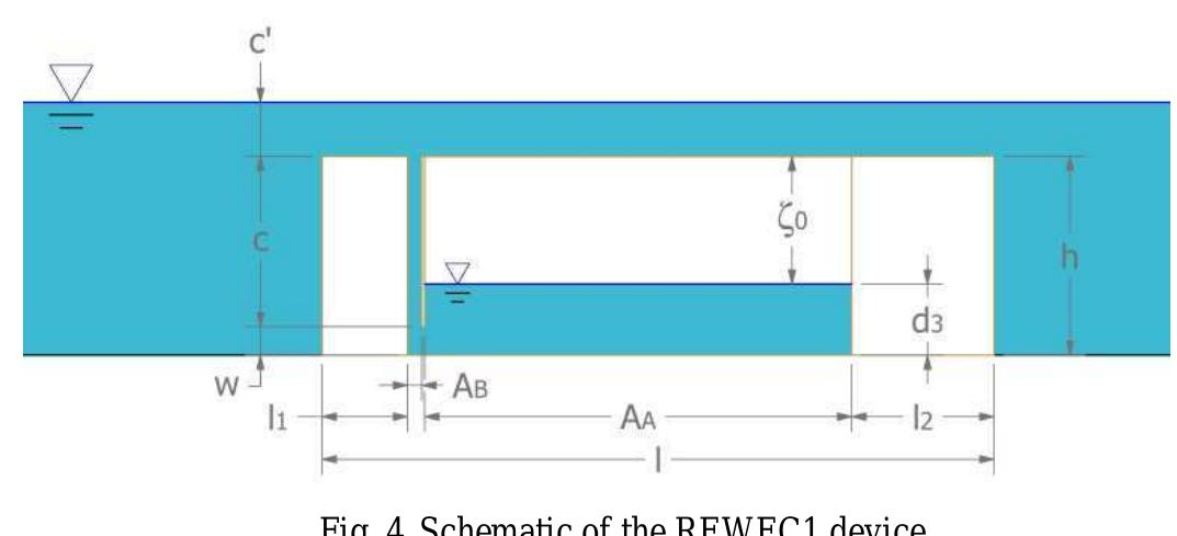
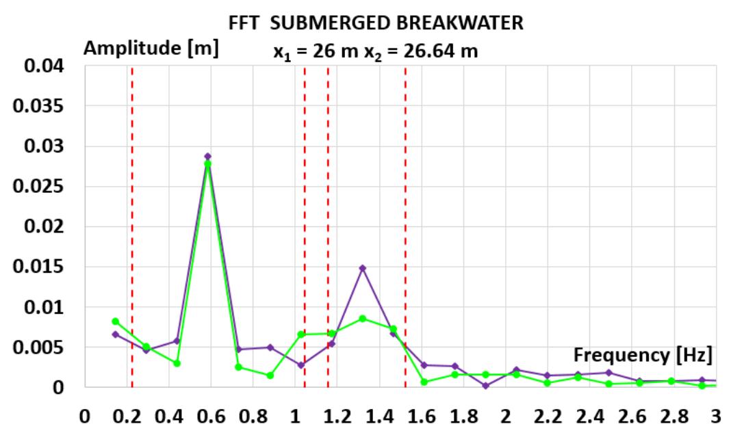
![Fig. 3 Schematic of the submerged impermeable breakwater of rectangular shape horizontal stretch (b, = 14.35 m in length) and then an inclined section (b; = 6.5 m in length) with a slope of 8.5°, simulating the presence of a shore. The submerged impermeable breakwater of rectangular shape has a length] = 2.36 m anda height h = 0.7 m, hence the submergence is c’= 0.2 m (Fig. 3).](https://figures.academia-assets.com/41855919/figure_003.jpg)
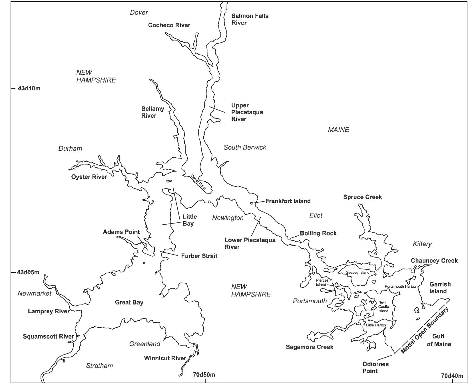
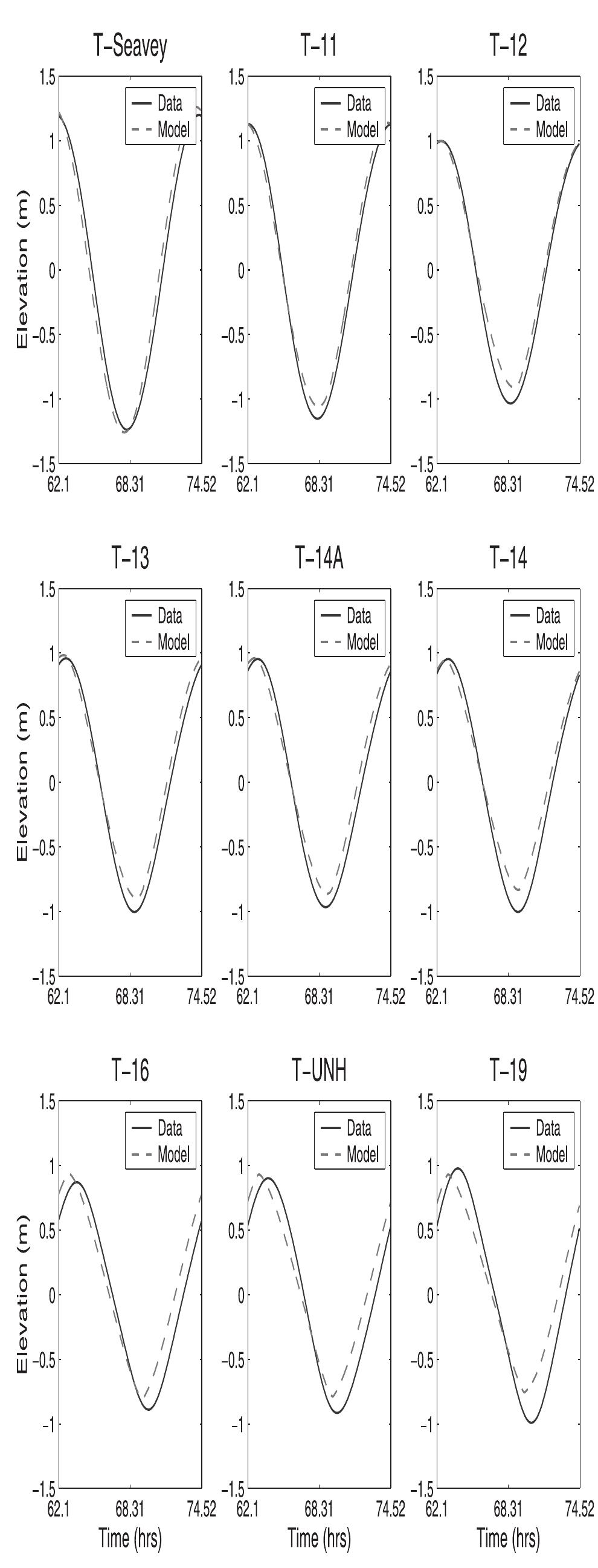
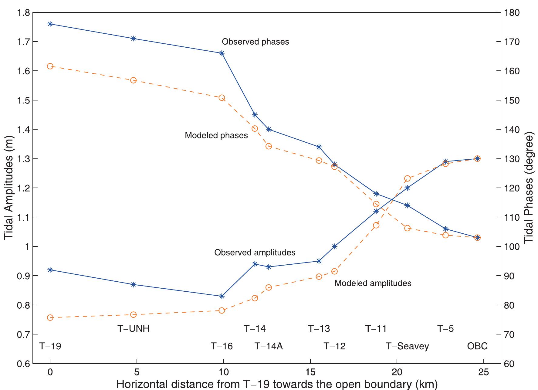
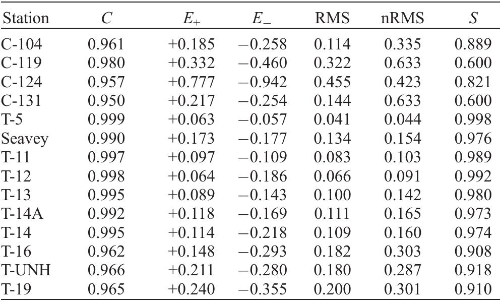
![Figure 3. Schematic geometry for the flooding and dewatering model [Ip et al., 1998]. at T-19 (Figure 2). The 76 deg M> phase lag of the T-19 Great Bay sea level relative to the open ocean boundary sea level explains most of the corresponding 2.5 hour time lag of total sea level. uent amplitude decreases from 1.29 m at the open ocean proxy station T-5 to 0.94 m (T-14) at the Dover Point confluence of the Lower Piscataqua, Upper Piscataqua, and Little Bay and increases throughout Little and Great Bays to the head of the inner estuary](https://figures.academia-assets.com/36476544/figure_003.jpg)
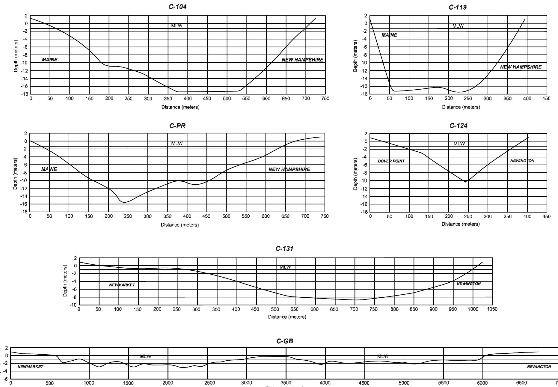
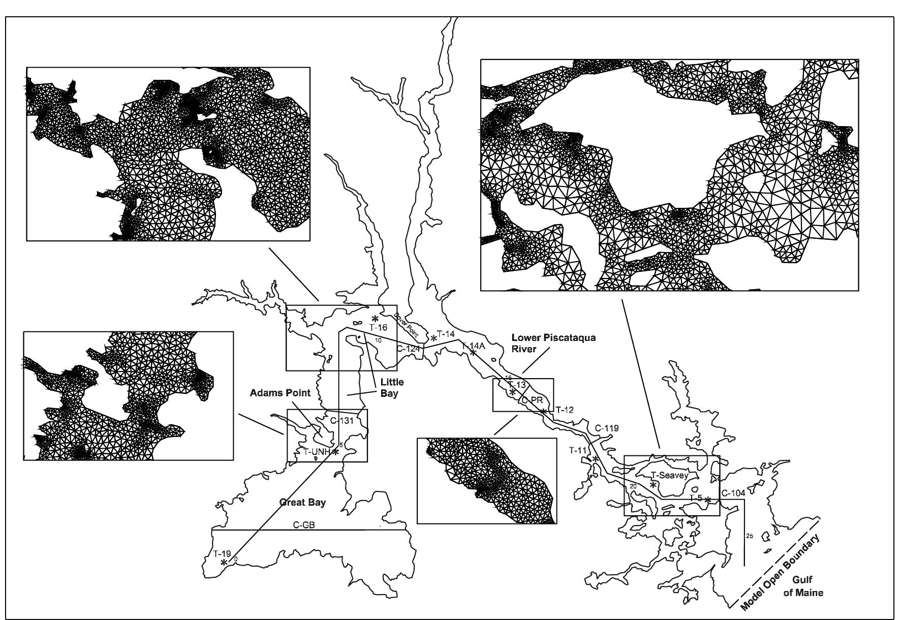
![Figure 5. Comparisons of M> amplitudes and Greenwich phases of surface elevations at the 10 observation stations. See color version of this figure at back of this issue. [15] Figure 2 displays example sections of the computational mesh (named gbesl0) that we constructed from available [13] Substituting the kinematic momentum balance into con- tinuity and incorporating the Darcian description for the porous medium sublayer, the governing equations for the composite](https://figures.academia-assets.com/36476544/figure_005.jpg)
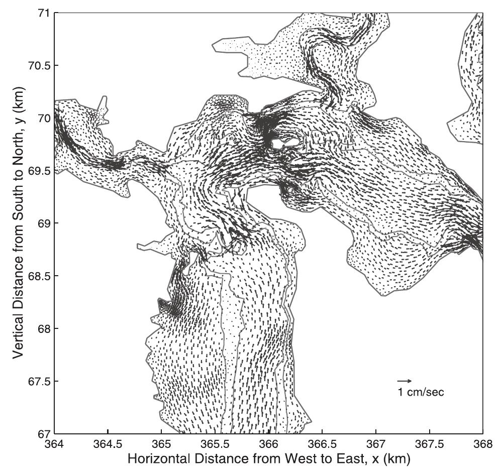
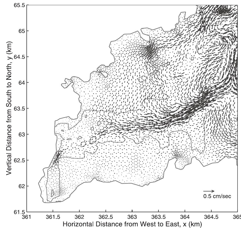
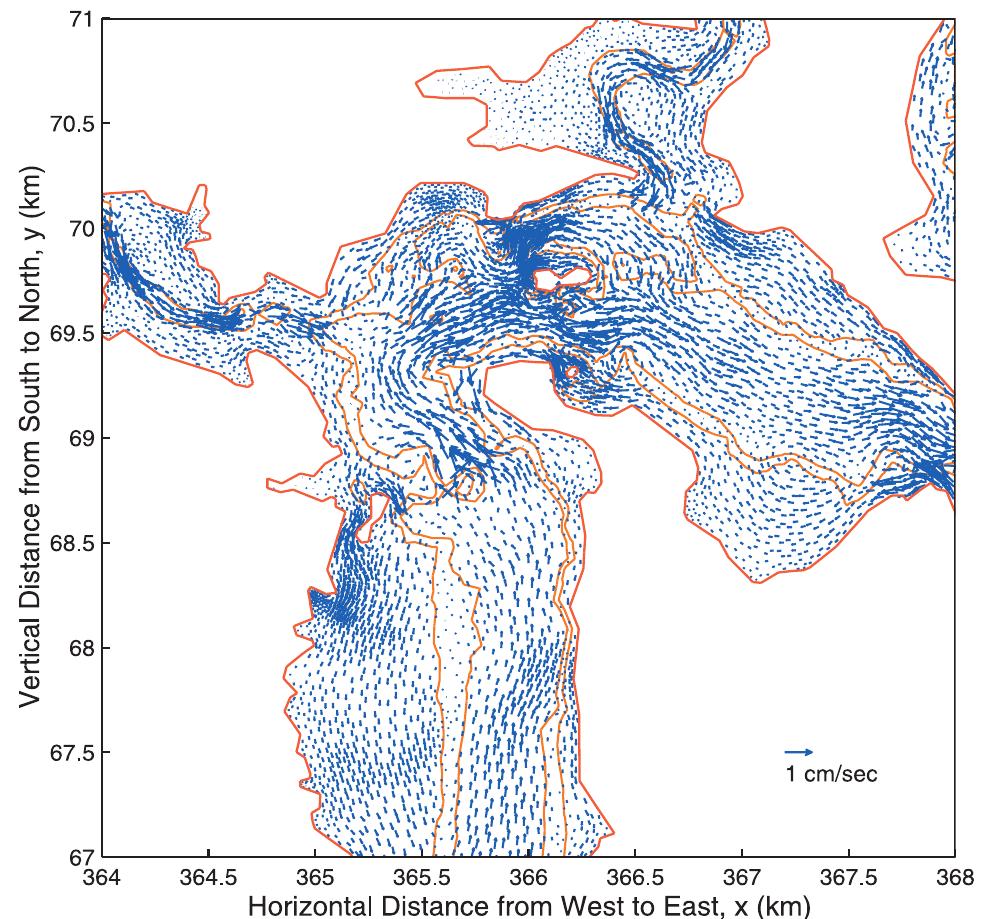
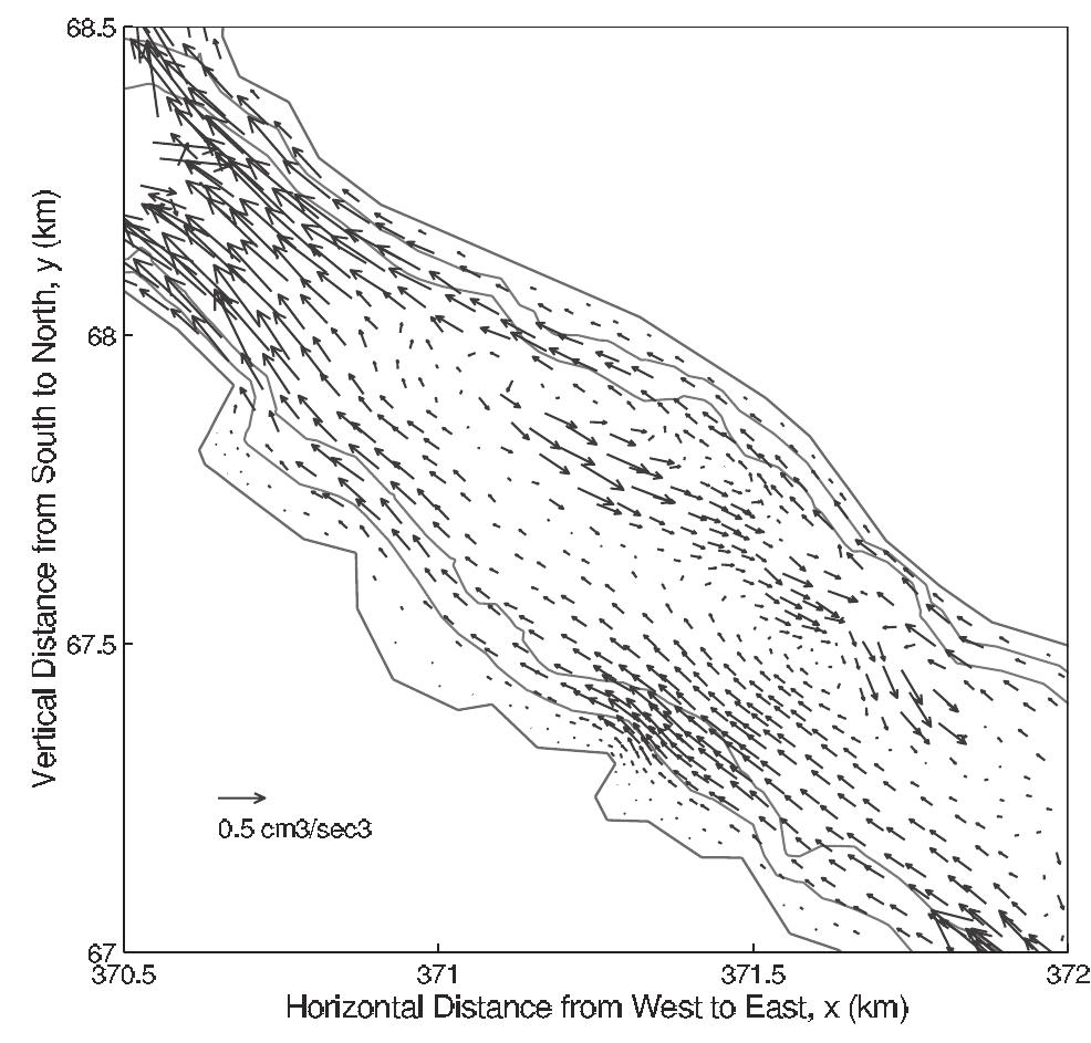
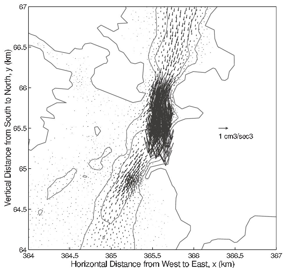
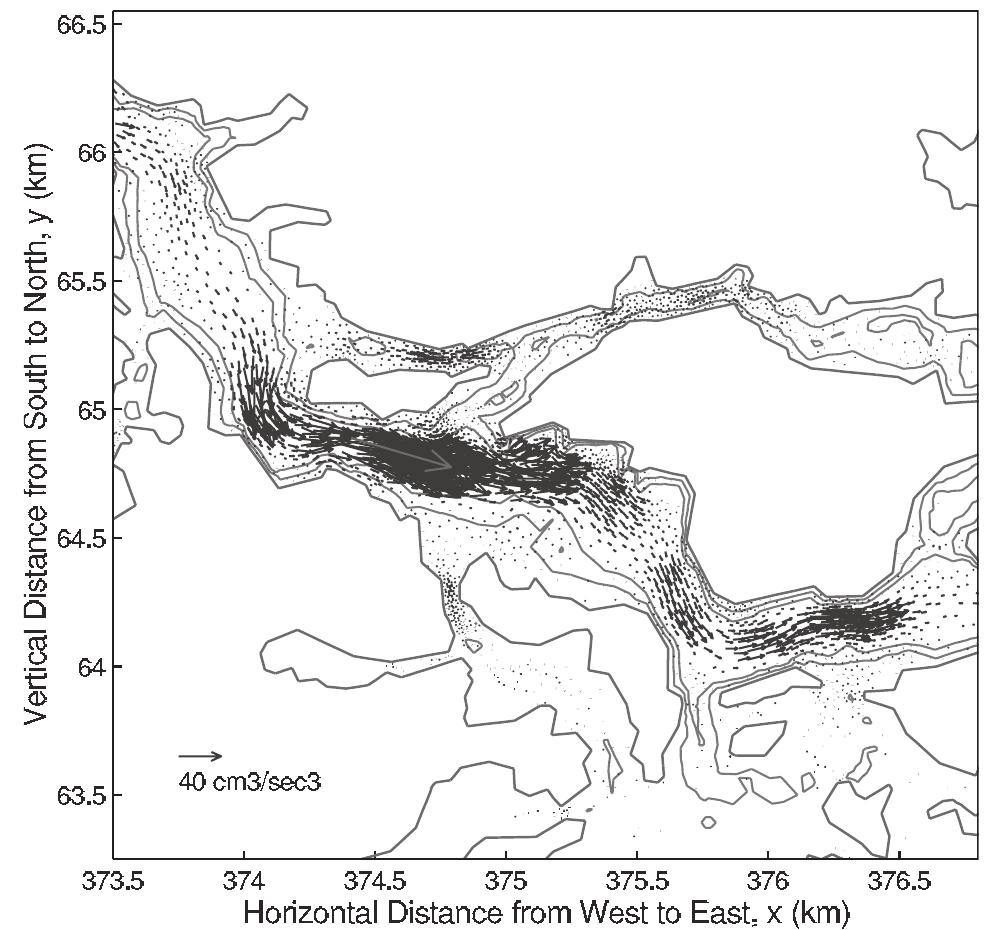
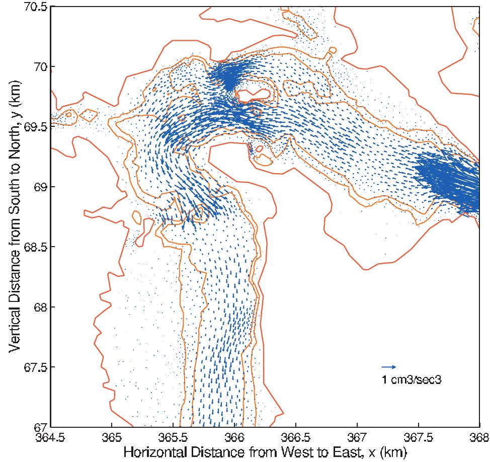
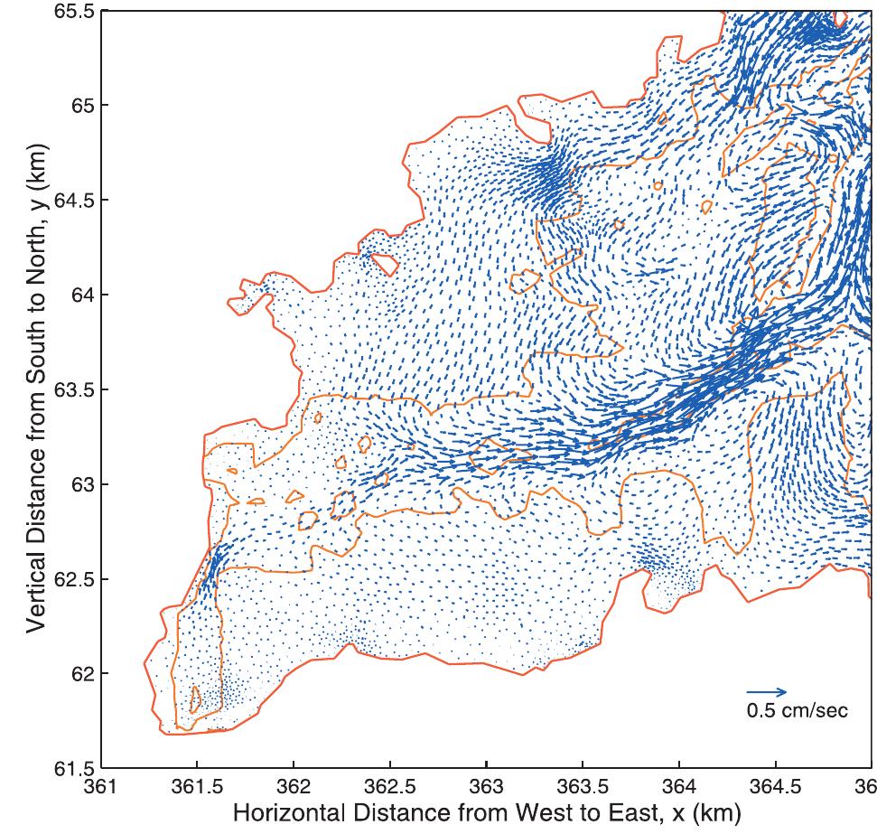
![Figure 10. Model residual sediment transport in Little Bay. See color version of this figure at back of this issue. [29] The landward transition from ebb to flood dominance may be due to the partially progressive nature of the tidal wave, which is characterized by flood currents at the crest (as well as ebb currents at the trough). Over shallow areas the flooding current at high water dominates since the low-water ebb is more restrained by bottom friction or may be missing altogether because of drying. The net volume transport into the estuary over the shallow boundary areas must then be balanced by outward residual current in the main channel. Similar situations have also been observed in other estuaries that are shallow with respect to their tidal range [see Friedrichs and Madsen, 1992; Bowers and Al-Barakati, 1997; Li and O'Donnell,](https://figures.academia-assets.com/36476544/figure_010.jpg)
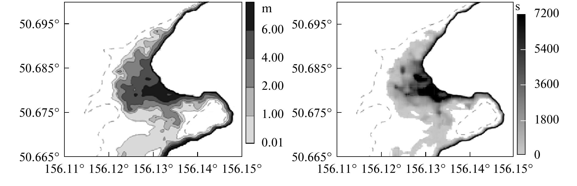
![Fig. 4. Comparison of flooded areas (shaded areas) in the second Kuril Strait in the vicinity of Severo-Kurilsk: field datz
on the tsunami of November 5, 1952 [21] (left) and numerical results (right).](https://figures.academia-assets.com/39627044/figure_006.jpg)